INTRODUCTION
This post shows how a simple virtual analog model / digital emulation of the first-order RC low-pass filter can be created using symbolic mathematics (i.e. computer algebra) in Python. The whole process is going to be automated and can be quickly adapted for modelling different, more complex linear audio circuitry. (Saves a lot of ink and paper.) I will leave it to the docs to explain all of the used functions in detail and concentrate more on the modelling part of things. A basic understanding of DSP is probably also necessary to understand everything mentioned here, but you can always check out things you are missing in any of the free books and tutorials available on the topic. This post is not meant to be an in-depth signal processing tutorial. Instead, you can see is as a sort of short introductory guide pointing in a few directions in case you are interested to learn more about modeling analog circuits.
Try running the notebook on your local machine or write the code yourself and check out the docs of the Python packages involved to get a better feel for the matter.
Code output is shown directly below the snippets.
PYTHON SETUP
Originally, all code was written in a Jupyter notebook, which is openly available on my GitHub (link). For this post I extracted the important lines and left out code that has only cosmetic purpose. Feel free to check out the notebook for the full code.
Creating our simple model requires us to have a few Python packages installed:
SymPy, a symbolic maths package, allowing us to do maths with symbols instead of concrete numerical values.
Lcapy, a symbolic circuit analysis toolkit built on SymPy, which we will use to draw a schematic and analyze the network.
Matplotlib.pyplot, a plotting library used to draw all function graphs.
NumPy, a numerical (as opposed so symbolic) maths package.
import sympy as sp # Symbolic maths
import lcapy as lp # Symbolic circuit analysis
import numpy as np # Numerical maths
import matplotlib.pyplot as plt # Plots and graphs
THE ANALOG MODEL
Before we can build a digital version of the RC low-pass filter it is necessary to analyze it in continuous time. We can use Lcapy to draw the schematic for us using a netlist specifying the electrical components and their connections. The netlist syntax is explained in great detail in the Lcapy docs. Drawing the circuit this way also allows for Lcapy to automatically analyze the schematic and find the transfer function for us later.
'''
Define the circuit through its netlist and draw schematic
'''

rclp1 = lp.Circuit("""
    P1 1 0; down, v=v_i
    R 1 2; right, R
    W  0 0_1; right
    C 2 0_1; down
    W 0_1 0_2; right
    W 2 2_1; right
    P2 2_1 0_2; down, v=v_o
""")

rclp1.draw()
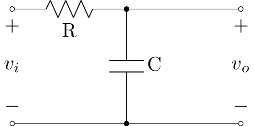
The analog transfer function $H(s)$ describing the circuit behaviour can be found in a single line of code. Output below is the transfer function in its symbolic form. Note that we have a formula in terms of ‘R’ and ‘C’ instead of concrete compenent values. With the help of SymPy we can now do all kinds of mathematical transformations, sort of like we would doing maths with pen and paper.
'''
Find analog transfer function specifying input and output ports as defined in the netlist
'''

Hs = rclp1.transfer('P1', 'P2').simplify()

sp.pretty_print(Hs)
H(s)=\frac{1}{C R s + 1}For our model we will express the filter in terms of the cutoff frequency, so we can ultimately expose the parameter in the algorithm. Of course, we can always revert the substitution at a later stage to design the filter by specifying raw component values (maybe you want to also model how component values change..). The (angular) cutoff frequency ($\omega_0$) $f_0$ is defined by:
\omega_0 = 2\pi f_0 = \frac{1}{RC}Rewriting the transfer function in terms of cutoff requires little coding effort. First we have to get a few symbols that were automatically created by Lcapy when finding the transfer function, as well as define one new smybol for the angular cutoff frequency. The Lcapy object is then converted into a regular SymPy expression that can then be further manipulated symbolically. Substituting in the cutoff is pretty straightforward. Because we are doing symbolic maths, it is necessary to use a symbolic representation of the number ‘1’ (sp.S.One) for the substitution. We will see later how it is possible to translate a symbolic expression into a function that, can be called with numerical values for the components.
'''
Rewrite H(s) in terms of the (angular) cutoff frequency w0
'''

# Get symbols from lcapy context for further calculations using sympy
C = lp.state.context.symbols.C
R = lp.state.context.symbols.R

# Define new symbol angular cutoff frequency
w0 = sp.symbols("omega0")

# Transform lcapy transfer function into regular sympy expression
Hs = Hs.sympy.simplify()

# Substitute
Hs = Hs.subs(R*C, sp.S.One / w0)

sp.pretty_print(Hs)
H(s)=\frac{1}{1 + \frac{s}{\omega_{0}}}
We have arrived at a mathematical decsription of the RC filter in the analog domain. Let’s now start the “virtual analog” part of the modeling process by deriving a discrete (digital) model from the analog one. Once we will have found the digital filter, we will plot and compare results.
BILINEAR TRANSFORMATION
To bring the analog filter we have just described into the digital domain, we will use a technique called bilinear transformation, which is a simple substitution of the Laplace $s$-variable (see Laplace transform). The bilinear transform is mapping of the imaginary frequency axis at $s=j\omega$ to the unit circle in the discrete $z$-plane (see z-transform).
s \leftarrow \frac{2}{T} \frac{z-1}{z+1}Because digital systems always have limited precision (finite number of bits) the mapping is unfortunately “not perfect”. Really only one frequency will be exactly preserved by the transformation and going off towards the extremes of the freqeuncy spectrum makes the digital model diverge more and more. Think of one interpretation as the infinitely long frequency axis of the $s$-plane getting skewed / squashed together to fit the not so infinite unit circle in the $z$-plane. (An effect known as “cramping”, which has also been center of a somewhat heated discussion on the web recently.) In Practice though, the mapping will be pretty accurate and only shows a large divergence closely to the Nyquist limit at the higher end of the frequency spectrum. A more closely matching model can be achieved by running the filter at a higher sample rate or by oversampling. (Other techniques exist, but those are left for a different day. Check the video linked above for more ideas on decramping digital filters.)
In the model we can freely choose the one frequency preserved by the mapping in a technique called prewarping. A useful choice would be to preserve the cutoff frequency, but your application may have restrictions requiring you to choose a different fixpoint. Prewarping results in a modified version of the standard bilinear transform substitution. This time we need to use a symbolic version of the tangent function (sp.tan()) instead of its regular numerical implementation.
'''
Define bilinear transformation with prewarping
'''

# Get some more symbols from lcapy context
s = lp.state.context.symbols.s
f = lp.state.context.symbols.f

# Define some more symbols
z = sp.symbols("z")
f0, T = sp.symbols("f0, T", real=True)

# Define the substitution with prewarping to preserve cutoff
blt = (w0 / sp.tan(w0 * T / 2)) * (z - 1) / (z + 1)

sp.pretty_print(blt)
s \leftarrow \frac{\omega_0}{\tan({\frac{\omega_o T}{2})}} \frac{z-1}{z+1}THE DIGITAL MODEL
The actual substitution can (once again) be done symbolically by means of a single line of code.
'''
Do the substitution to find the digital model
'''

Hz = Hs.subs(s, blt).simplify()

sp.pretty_print(Hz)
H(z) = \frac{\left(z + 1\right) \tan{\left(\frac{T \omega_{0}}{2} \right)}}{z + \left(z + 1\right) \tan{\left(\frac{T \omega_{0}}{2} \right)} - 1}And there we have it – our digital filter, analog modeled. The SymPy output, though mathematically correct, does not always look the way we would have written it by hand, but there are many functions to express a formula in different ways which we could try to make things look nicer (check the docs for an extensive introduction). Luckily for us, SymPy does not care too much about the looks of mathematical expressions and we can safely continue our modeling endeavour without worrying about this for now.
Because $\tan{x}\approx x$ for small values of $x$, we can further simplify the calculation omitting the computanionally costful tangent functions entirely. We know that the argument of the tangent functions stays “small enough” for this to not distort the amplitude repsonse too much.
'''
Simplify H(z) for more efficient implementation
'''

Hz = Hz.subs(sp.tan(w0*T/2), w0*T/2).simplify()

sp.pretty_print(Hz)
H(z) = \frac{T \omega_{0} \left(z + 1\right)}{T \omega_{0} \left(z + 1\right) + 2 z - 2}All that’s left to do now is extract the filter coefficients and we are done with the model, ready to implement the filter digitally.
The coefficients are named according to:
H(z) = \frac{a_0 + a_1 z^{-1}}{1 + b_1 z^{-1}}(Note that coeffficient $b_0$ is normalized to 1.)
'''
Find discrete filter coefficients
'''

# Get numerator / denominator
num, den = Hz.as_numer_denom()

# Extract coefficient arrays
numCoeffs = num.as_expr().as_poly(z).simplify().coeffs()
denCoeffs = den.as_expr().as_poly(z).simplify().coeffs()

# Normalize coefficient b0 to 1 (divide all coeffs by b0)

b0 = denCoeffs[0]

numCoeffsNorm = []
denCoeffsNorm = []

for coeff in numCoeffs:
    coeff /= b0
    numCoeffsNorm.append(coeff)
for coeff in denCoeffs:
    coeff /= b0
    denCoeffsNorm.append(coeff)

print("a0: ", numCoeffsNorm[0])
print("a1: ", numCoeffsNorm[1])
print("b0: ", denCoeffsNorm[0])
print("b1: ", denCoeffsNorm[1])
a0:  T*omega0/(T*omega0 + 2)
a1:  T*omega0/(T*omega0 + 2)
b0:  1
b1:  (T*omega0 - 2)/(T*omega0 + 2)
Voilà – The coefficients of our virtual analog filter!
These can now be used to, for instance, filter a signal in real-time inside of an audio plugin or similar application.
All that’s necessary is to implement the difference equation to do time domain filtering. Here $y[n]$ describes the output samples and $x[n]$ describes input samples at timestep $n$. The current output sample can be found as a (discrete) function of current, as well as previous, input and output samples (see IIR filters). (If it’s not obvious, $n-1$ refers to a one-sample delay.) The difference equation is found by means of the inverse z-transform.
y[n] = a_0 x[n] + a_1 x[n-1] - b_1 y[n-1]
MODEL COMPARISON
To conclude, let’s plot and compare the two models. We will first transform the symbolic expressions of both transfer functions into a numerical function, that we can input concrete frequency (component) values in a process called “lambdification”. Magnitude and phase response of the analog filter can then be found by evaluating $H(s)$ at $s=j\omega$. For the digital filter we will instead evaluate $H(z)$ at $z=e^{j\omega T}$.
'''
Evaluate frequency responses to find magnitude and phase
'''

# ANALOG

# Create frequency vector
fVals = 20 * np.logspace(0, 3, 300) # 20Hz - 20kHz

# Evaluate the analog transfer function at s=jw to find the frequency response
sSub = 1j * 2 * np.pi * f
HsEval = HsEval.subs(s, sSub)

# Make Hs a callable function, so numpy arrays work as input
Hs_f = sp.lambdify(f, HsEval, "numpy") # H_s(f)

# Find magnitude and phase
sFreqResp = Hs_f(fVals)
sMag = 20 * np.log10(np.abs(sFreqResp))
sPhase = np.angle(sFreqResp)

# DIGITAL

# Make Hs a callable function, so numpy arrays work as input
Hz_f = sp.lambdify(z, HzEval, "numpy")

# Evaluate the digital transfer function at z = exp(jwT) to find the frequency response
zSub = np.exp(1j * 2 * np.pi * fVals * TVal)
zFreqResp = Hz_f(zSub)

# Find magnitude and phase
zMag = 20 * np.log10(np.abs(zFreqResp))
zPhase = np.angle(zFreqResp)
Now, a Bode plot can be created with Matplotlib.
# Create Bode plot
fig, ax = plt.subplots(2, 1, sharex=False, sharey=False, figsize=(4.5, 3))
print(f"(fs = {fsVal: 1.0f} Hz)")

ax[0].yaxis.set_major_formatter(ticker.FormatStrFormatter(r'%.1f'))
ax[1].yaxis.set_major_formatter(ticker.FormatStrFormatter(r'%.1f $\pi$'))

ax[0].semilogx(fVals, sMag, label="Analog")
ax[0].semilogx(fVals, zMag, label=r"Digital (48kHz)")
ax[0].set_ylabel("Magnitude / dB")
ax[0].legend()

ax[1].semilogx(fVals, zPhase)
ax[1].semilogx(fVals, sPhase)
ax[1].set_xlabel("Frequency / Hz")
ax[1].set_ylabel("Phase / rad")

# Draw Nyquist limit as vertical, dashed lines
ax[0].vlines(fsVal / 2, -50, 0, color="lightgrey", linestyle="dashed")
ax[1].vlines(fsVal / 2, -1.5, 0, color="lightgrey", linestyle="dashed")

plt.tight_layout()
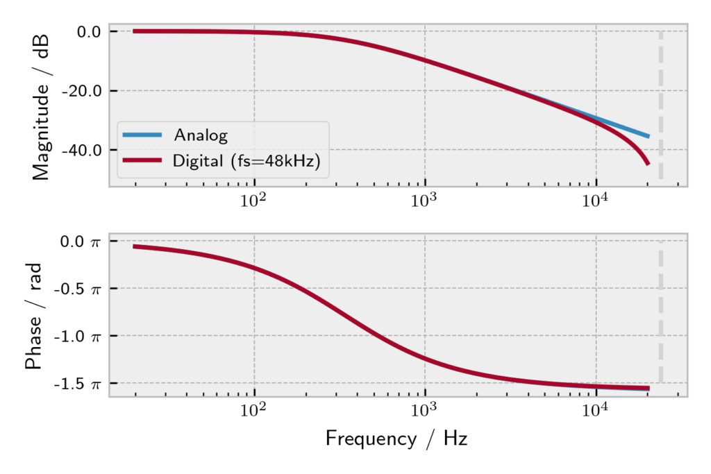
As expected, the models are an almost perfect fit, except for the cramping that shows at frequencies near $f_s / 2$. (Try running the notebook at a higher sample rate like 96 kHz and see how the curves change. (Hint: The curves will match almost exactly all the way up to 20 kHz.) Moving the Nyguist limit higher also makes the cramping appear at higher frequencies, where it quickly becomes inaudible.
Of course, discretizing a one-pole RC filter it is not the most interesting project in terms of analog modeling, but the techniques presented here can be used to model more complex filters. The whole process gets rather difficult for systems of order 3 or higher, especially those with many loops and components. Such systems will require us to symbolically handle large expressions with many coefficients and difference equations of higher order can lead to numerical problems. If possible, higher order filters should be split into a cascade of second-order stages before even designing the digital filter. I will probably write about a more “real world” type of model sometime in the future. I hope, that I was nonetheless able to give a short but interesting glimpse into the modeling process.
If you want to learn more about virtual analog filters – In my opinion there is no better book than Vadim Zavalishin’s “The Art of VA Filter Design”. You can download it freely here (Native Instruments website).